Phyloseq BUG Meeting Presentation Fall 2019
Introduction
Dataset examined is from this file https://www.mothur.org/MiSeqDevelopmentData/StabilityNoMetaG.tar
The full MiSeqSOP, a partial dataset is discussed here on the mothur website: https://www.mothur.org/wiki/MiSeq_SOP
Here is a small excerpt from the site that describes the study design:
Starting out we need to first determine, what is our question? The Schloss lab
is interested in understanding the effect of normal variation in the gut
microbiome on host health. To that end we collected fresh feces from mice on a
daily basis for 365 days post weaning (we're accepting applications). During the
first 150 days post weaning (dpw), nothing was done to our mice except allow
them to eat, get fat, and be merry. We were curious whether the rapid change in
weight observed during the first 10 dpw affected the stability microbiome
compared to the microbiome observed between days 140 and 150.
NOTE: BECAUSE THIS DATA IS TIME SERIES, THE STATISTICAL TESTS SHOWN BELOW ARE INCORRECT. I’VE DONE THIS BECAUSE MANY PEOPLE WILL NOT HAVE TIME-COURSE DATA AND THEREFORE THE PAIRED STATISTICAL TESTS ARE LESS REPRESENTATIVE OF ACTUAL DATA ANALYSIS
If you have time-series data, then you MUST make sure you are using the paired statistical tests.
Let’s import some data that we previously generated using dada2.
base <- here('content', 'posts', 'data',
     '2019-11-06-phyloseq-bug-meeting-presentation-fall-2019')
metadata <- read.table(file.path(base, 'metadata.tab'), sep='\t', header = T,
                       colClasses = c('character', 'factor', 'factor',
                                      'numeric', 'factor'))
seqtab.nochim <- readRDS(file.path(base, "seqtab_nochim.rds"))
seqtab.taxa <- readRDS(file.path(base, "tax.rds"))
rownames(metadata) <- metadata$sample

#Get ordering to preserve data presentation order throughout analysis
colnames(metadata)
## [1] "sample" "mouse" "sex" "day" "time"# metadata$time
primary <- 'time'
primary_order_list <- c('early', 'midearly', 'mid', 'late', 'post')
metadata$time <- factor(metadata$time, levels = primary_order_list)
levels(metadata$time)## [1] "early" "midearly" "mid" "late" "post"# metadata$sex
secondary <- 'sex'
secondary_order_list <- c('female', 'male')
metadata$sex <- factor(metadata$sex, levels = secondary_order_list)
levels(metadata$sex)## [1] "female" "male"# Get color list
ncolors <- length(levels(metadata$time))
primary_color_list <- brewer.pal(ncolors, 'Dark2')
#Convert to phyloseq object
ps <- phyloseq(otu_table(seqtab.nochim, taxa_are_rows=FALSE),
sample_data(metadata),
tax_table(seqtab.taxa))
#convert names to arbitrary ASV names
names.ps <- as.data.frame(cbind(taxa_names(ps),
paste0("ASV", seq(ntaxa(ps)))),
stringsAsFactors=F)
colnames(names.ps) <- c('seq', 'asv')
taxa_names(ps) <- names.ps$asvLet’s explore the data a bit before we do any diversity plots
ps## phyloseq-class experiment-level object
## otu_table() OTU Table: [ 403 taxa and 360 samples ]
## sample_data() Sample Data: [ 360 samples by 5 sample variables ]
## tax_table() Taxonomy Table: [ 403 taxa by 7 taxonomic ranks ]observed <- estimate_richness(ps, measures = c('Observed'))
explore.df <- cbind(observed, sample_sums(ps), sample_data(ps)$time)
colnames(explore.df) <- c('Observed', 'Sample_Sums', 'Time')
observed_mean <- mean(explore.df$Observed)
sample_sum_mean <- mean(explore.df$Sample_Sums)
ggplot(data = explore.df, aes(x = Sample_Sums, y = Observed, color = Time)) +
geom_point() +
geom_smooth(method="auto", se=TRUE, fullrange=FALSE, level=0.95,
inherit.aes = F, mapping = aes(Sample_Sums, Observed),
data = explore.df) +
scale_color_manual(values = primary_color_list)## `geom_smooth()` using method = 'loess' and formula 'y ~ x'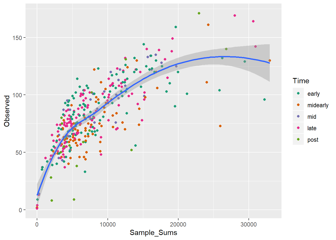
# Let's use ampvis2 again so we can easily make a rarefaction curve

# Need to convert from phyloseq to ampvis
av2_otutable <- data.frame(OTU = rownames(t(phyloseq::otu_table(ps)@.Data)),
                       t(phyloseq::otu_table(ps)@.Data),
                       phyloseq::tax_table(ps)@.Data,
                       check.names = F
)

#Extract metadata from the phyloseq object:
av2_metadata <- data.frame(phyloseq::sample_data(ps),
                       check.names = F
)

av2_metadata <- cbind(rownames(av2_metadata), av2_metadata)

#Load the data with amp_load:
av2_obj <- amp_load(av2_otutable, av2_metadata)

# RARE CURVE
rare_plot_amp <- amp_rarecurve(data = av2_obj, color_by = primary)
rare_curve_plot <- rare_plot_amp + ylab('Observed ASVs (count)') +
  # geom_vline(xintercept=min(sample_sums(ps2)), linetype='dashed') +
  scale_color_manual(values =  primary_color_list) +
  xlim(c(0, 35000))
rare_curve_plot
sort(explore.df$Sample_Sums)## [1] 1 10 11 19 75 254 268 697 734 788 1184
## [12] 1449 1938 1970 1984 2069 2070 2108 2164 2185 2284 2350
## [23] 2380 2507 2561 2746 2782 2803 2844 2918 2936 2952 2975
## [34] 3090 3092 3100 3105 3172 3278 3319 3367 3380 3433 3452
## [45] 3483 3515 3547 3576 3630 3658 3660 3710 3711 3730 3752
## [56] 3755 3765 3771 3776 3782 3819 3856 3877 3877 3889 3894
## [67] 3897 3908 3931 3932 3997 4028 4078 4088 4095 4113 4131
## [78] 4187 4205 4210 4231 4250 4259 4275 4329 4366 4405 4414
## [89] 4419 4430 4456 4475 4514 4517 4529 4562 4583 4640 4641
## [100] 4653 4660 4660 4685 4707 4727 4728 4734 4735 4791 4814
## [111] 4850 4860 4890 4908 4942 4984 4986 5038 5043 5079 5117
## [122] 5122 5124 5182 5200 5214 5215 5240 5240 5243 5250 5263
## [133] 5270 5359 5381 5396 5418 5472 5489 5492 5507 5540 5541
## [144] 5617 5657 5662 5694 5695 5700 5771 5835 5855 5876 5930
## [155] 6024 6028 6028 6029 6052 6087 6098 6139 6153 6187 6224
## [166] 6270 6352 6463 6550 6554 6580 6584 6599 6632 6642 6665
## [177] 6685 6726 6761 6786 6810 6814 6830 6847 6854 6855 6861
## [188] 6865 6897 6912 7008 7046 7135 7207 7219 7223 7244 7268
## [199] 7326 7428 7458 7463 7566 7566 7588 7599 7672 7739 7761
## [210] 7782 7786 7813 7875 7882 7926 7992 8057 8058 8088 8091
## [221] 8108 8118 8154 8178 8286 8358 8362 8403 8525 8540 8658
## [232] 8661 8751 8843 8912 8960 8966 9048 9067 9073 9145 9320
## [243] 9378 9480 9504 9526 9550 9565 9714 9782 9981 10067 10106
## [254] 10119 10169 10179 10350 10358 10451 10533 10620 10630 10667 10713
## [265] 10726 10761 10763 11143 11163 11222 11226 11253 11266 11349 11412
## [276] 11534 11535 11581 11600 11741 11912 11944 12007 12084 12118 12125
## [287] 12225 12226 12424 12475 12488 12496 12510 12539 12571 12577 12703
## [298] 12745 12761 12807 12984 13383 13462 13779 13809 13948 13998 14085
## [309] 14108 14278 14433 14484 14616 14716 14883 15104 15171 15198 15212
## [320] 15310 15485 15549 15668 15920 16057 16138 16215 16279 16621 16812
## [331] 16859 16885 17027 17283 17625 17708 18135 18350 18461 18797 19063
## [342] 19181 19531 19632 19733 19958 21235 22927 24018 24239 25839 25943
## [353] 26225 26804 27999 29429 30626 30932 32226 32963summary(explore.df$Sample_Sums)## Min. 1st Qu. Median Mean 3rd Qu. Max.
## 1 4450 6798 8413 11223 32963length(explore.df$Sample_Sums)## [1] 360length(which(explore.df$Sample_Sums < 2500))## [1] 23rare_curve_plot + geom_vline(xintercept = 2500, linetype = 'dashed')
# remove samples below 2500 total reads
ps_sub <- subset_samples(ps, sample_sums(ps) > 2500)
We’ve removed samples with fewer than 2500 reads. Now, lets calculate some diversity values.
plot_richness(ps_sub, measures = c('Shannon', 'Simpson'))## Warning in estimate_richness(physeq, split = TRUE, measures = measures): The data you have provided does not have
## any singletons. This is highly suspicious. Results of richness
## estimates (for example) are probably unreliable, or wrong, if you have already
## trimmed low-abundance taxa from the data.
##
## We recommended that you find the un-trimmed data and retry.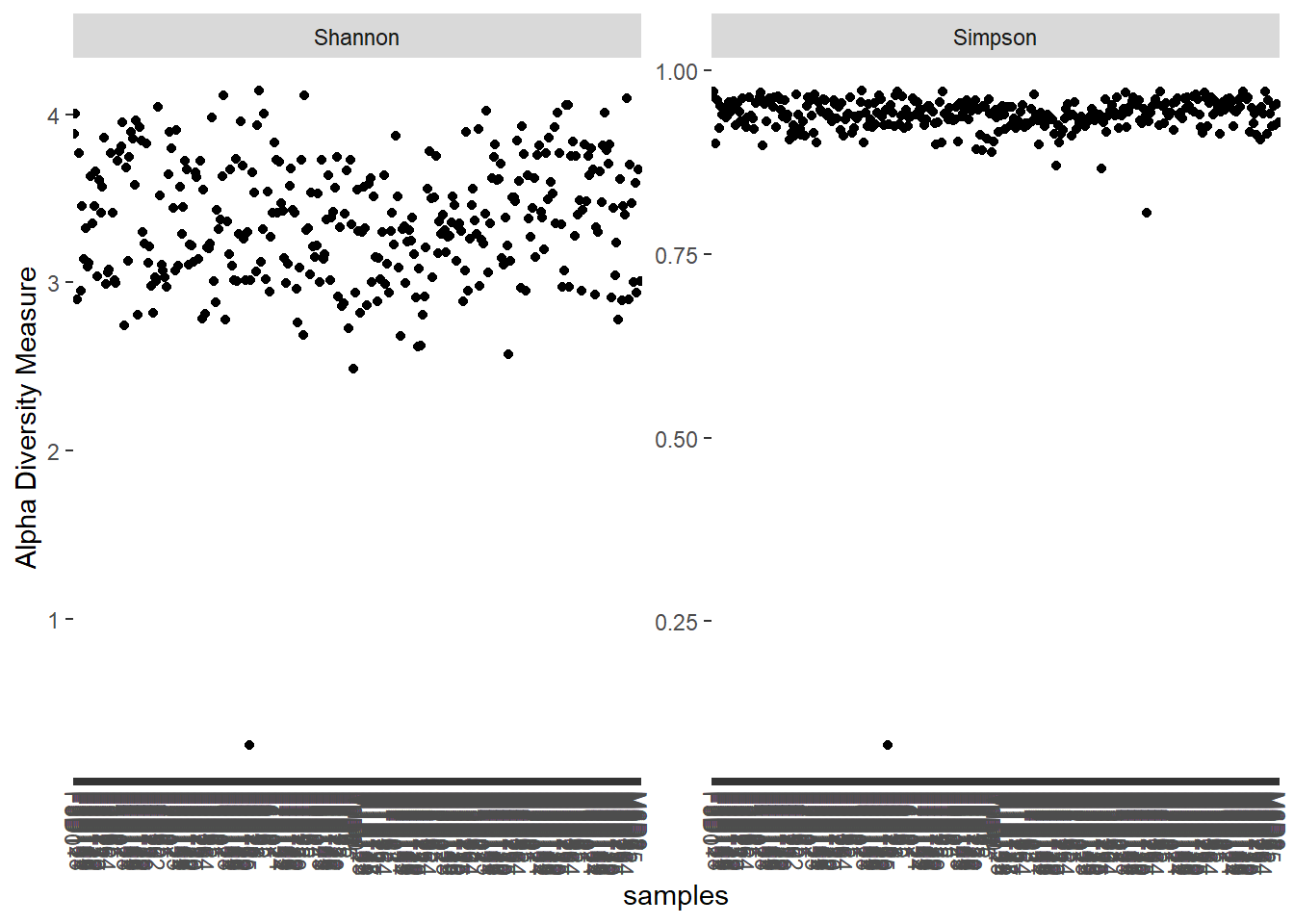
ps_sub.rare <- rarefy_even_depth(ps_sub)## You set `rngseed` to FALSE. Make sure you've set & recorded
## the random seed of your session for reproducibility.
## See `?set.seed`## ...## 11OTUs were removed because they are no longer
## present in any sample after random subsampling## ...sample_sums(ps_sub.rare)## F3D0 F3D1 F3D11 F3D125 F3D13 F3D141 F3D142 F3D143 F3D144 F3D145
## 2507 2507 2507 2507 2507 2507 2507 2507 2507 2507
## F3D146 F3D147 F3D148 F3D149 F3D15 F3D150 F3D17 F3D2 F3D21 F3D25
## 2507 2507 2507 2507 2507 2507 2507 2507 2507 2507
## F3D3 F3D364 F3D5 F3D6 F3D65 F3D7 F3D8 F3D9 F4D0 F4D1
## 2507 2507 2507 2507 2507 2507 2507 2507 2507 2507
## F4D11 F4D125 F4D13 F4D141 F4D142 F4D143 F4D144 F4D145 F4D146 F4D147
## 2507 2507 2507 2507 2507 2507 2507 2507 2507 2507
## F4D148 F4D149 F4D15 F4D150 F4D17 F4D19 F4D2 F4D21 F4D25 F4D3
## 2507 2507 2507 2507 2507 2507 2507 2507 2507 2507
## F4D302 F4D4 F4D5 F4D6 F4D65 F4D7 F4D8 F4D9 F5D0 F5D1
## 2507 2507 2507 2507 2507 2507 2507 2507 2507 2507
## F5D11 F5D125 F5D13 F5D141 F5D142 F5D143 F5D144 F5D146 F5D147 F5D148
## 2507 2507 2507 2507 2507 2507 2507 2507 2507 2507
## F5D149 F5D15 F5D150 F5D17 F5D19 F5D2 F5D21 F5D25 F5D3 F5D364
## 2507 2507 2507 2507 2507 2507 2507 2507 2507 2507
## F5D4 F5D45 F5D5 F5D6 F5D65 F5D7 F5D8 F5D9 F6D0 F6D1
## 2507 2507 2507 2507 2507 2507 2507 2507 2507 2507
## F6D11 F6D125 F6D13 F6D141 F6D142 F6D143 F6D144 F6D145 F6D146 F6D147
## 2507 2507 2507 2507 2507 2507 2507 2507 2507 2507
## F6D148 F6D149 F6D15 F6D150 F6D165 F6D17 F6D19 F6D2 F6D21 F6D25
## 2507 2507 2507 2507 2507 2507 2507 2507 2507 2507
## F6D3 F6D4 F6D45 F6D5 F6D6 F6D65 F6D7 F6D8 F6D9 F7D0
## 2507 2507 2507 2507 2507 2507 2507 2507 2507 2507
## F7D1 F7D11 F7D124 F7D13 F7D141 F7D142 F7D143 F7D144 F7D145 F7D146
## 2507 2507 2507 2507 2507 2507 2507 2507 2507 2507
## F7D147 F7D148 F7D149 F7D15 F7D150 F7D2 F7D25 F7D3 F7D4 F7D45
## 2507 2507 2507 2507 2507 2507 2507 2507 2507 2507
## F7D5 F7D6 F7D65 F7D7 F7D9 F8D0 F8D1 F8D125 F8D141 F8D142
## 2507 2507 2507 2507 2507 2507 2507 2507 2507 2507
## F8D143 F8D144 F8D145 F8D146 F8D147 F8D148 F8D150 F8D2 F8D25 F8D3
## 2507 2507 2507 2507 2507 2507 2507 2507 2507 2507
## F8D4 F8D45 F8D5 F8D6 F8D65 F8D7 F8D8 F8D9 M1D0 M1D1
## 2507 2507 2507 2507 2507 2507 2507 2507 2507 2507
## M1D11 M1D125 M1D13 M1D142 M1D143 M1D144 M1D145 M1D147 M1D148 M1D15
## 2507 2507 2507 2507 2507 2507 2507 2507 2507 2507
## M1D17 M1D19 M1D21 M1D25 M1D3 M1D364 M1D4 M1D5 M1D6 M1D65
## 2507 2507 2507 2507 2507 2507 2507 2507 2507 2507
## M1D8 M2D0 M2D1 M2D11 M2D13 M2D141 M2D142 M2D143 M2D144 M2D145
## 2507 2507 2507 2507 2507 2507 2507 2507 2507 2507
## M2D146 M2D147 M2D148 M2D149 M2D15 M2D150 M2D17 M2D2 M2D21 M2D25
## 2507 2507 2507 2507 2507 2507 2507 2507 2507 2507
## M2D3 M2D364 M2D4 M2D5 M2D6 M2D65 M2D7 M2D8 M2D9 M3D0
## 2507 2507 2507 2507 2507 2507 2507 2507 2507 2507
## M3D11 M3D125 M3D13 M3D142 M3D143 M3D144 M3D145 M3D146 M3D15 M3D150
## 2507 2507 2507 2507 2507 2507 2507 2507 2507 2507
## M3D17 M3D175 M3D19 M3D2 M3D21 M3D25 M3D364 M3D4 M3D45 M3D6
## 2507 2507 2507 2507 2507 2507 2507 2507 2507 2507
## M3D65 M3D7 M3D9 M4D0 M4D11 M4D125 M4D13 M4D141 M4D142 M4D143
## 2507 2507 2507 2507 2507 2507 2507 2507 2507 2507
## M4D144 M4D145 M4D146 M4D147 M4D149 M4D15 M4D150 M4D17 M4D175 M4D19
## 2507 2507 2507 2507 2507 2507 2507 2507 2507 2507
## M4D2 M4D21 M4D25 M4D3 M4D364 M4D4 M4D45 M4D5 M4D6 M4D65
## 2507 2507 2507 2507 2507 2507 2507 2507 2507 2507
## M4D7 M4D8 M4D9 M5D0 M5D1 M5D11 M5D124 M5D13 M5D141 M5D142
## 2507 2507 2507 2507 2507 2507 2507 2507 2507 2507
## M5D143 M5D144 M5D145 M5D146 M5D147 M5D148 M5D149 M5D15 M5D150 M5D17
## 2507 2507 2507 2507 2507 2507 2507 2507 2507 2507
## M5D175 M5D19 M5D2 M5D21 M5D25 M5D3 M5D364 M5D4 M5D45 M5D5
## 2507 2507 2507 2507 2507 2507 2507 2507 2507 2507
## M5D6 M5D65 M5D7 M5D8 M5D9 M6D0 M6D1 M6D11 M6D124 M6D13
## 2507 2507 2507 2507 2507 2507 2507 2507 2507 2507
## M6D141 M6D142 M6D143 M6D144 M6D145 M6D146 M6D147 M6D148 M6D149 M6D15
## 2507 2507 2507 2507 2507 2507 2507 2507 2507 2507
## M6D150 M6D17 M6D175 M6D19 M6D2 M6D21 M6D25 M6D3 M6D364 M6D4
## 2507 2507 2507 2507 2507 2507 2507 2507 2507 2507
## M6D45 M6D5 M6D6 M6D65 M6D7 M6D8 M6D9
## 2507 2507 2507 2507 2507 2507 2507plot_richness(ps_sub.rare, measures = c('Shannon', 'Simpson'))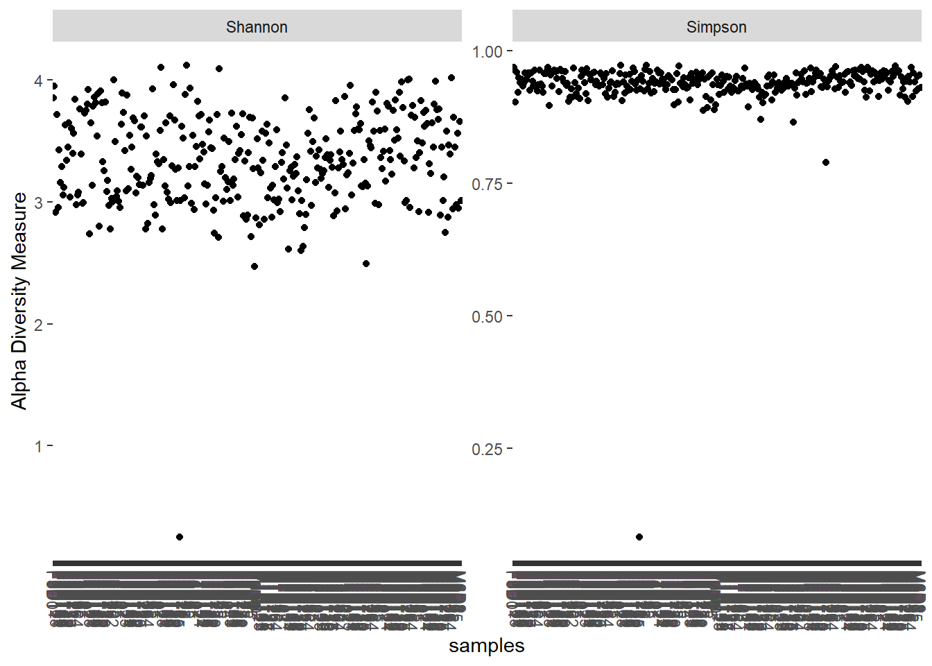
richness.rare <- cbind(estimate_richness(ps_sub.rare,
                                         measures = c('Shannon', 'Simpson')),
                       sample_data(ps_sub.rare)$time)
colnames(richness.rare) <- c('Shannon', 'Simpson', 'Time')
richness.rare$Labels <- rownames(richness.rare)

ggplot(data = richness.rare, aes(x = Shannon, y = Simpson)) +
  geom_point()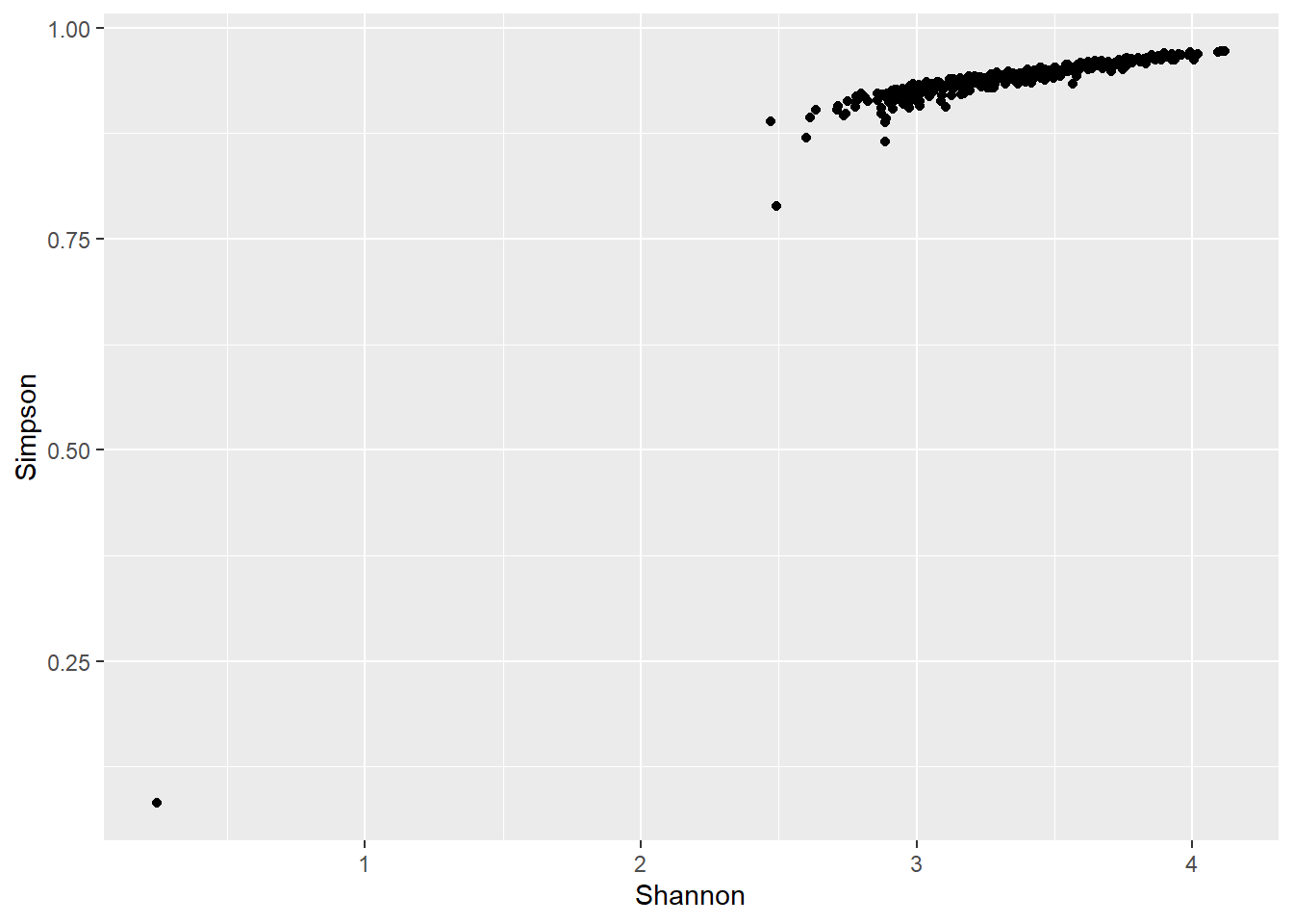
message('Simpson index as returned by vegan package is 1-D, rather than D itself.')## Simpson index as returned by vegan package is 1-D, rather than D itself.ggplot(data = richness.rare, aes(x = Shannon, y = (Simpson-1)*-1, color = Time)) +
geom_point() +
# geom_smooth(method="auto", se=TRUE, fullrange=FALSE, level=0.95,
# inherit.aes = F, mapping = aes(Shannon, Simpson),
# data = richness.rare) +
scale_color_manual(values = primary_color_list) +
geom_text(aes(label=ifelse(Shannon<1, Labels, ""), hjust=-0.1),
show.legend = F) +
xlim(c(0,max(richness.rare$Shannon))) +
theme_cowplot()
outlier <- data.frame(otu_table(ps_sub.rare)['F6D165',])
outlier <- reshape2::melt(outlier)
## No id variables; using all as measure variablesoutlier[order(outlier$value, decreasing = T),][1:10,]## variable value
## 13 ASV13 2402
## 227 ASV227 38
## 134 ASV134 24
## 109 ASV109 11
## 146 ASV146 11
## 206 ASV206 9
## 315 ASV315 8
## 3 ASV3 3
## 5 ASV5 1
## 1 ASV1 0richness.rare['F6D165',]## Shannon Simpson Time Labels
## F6D165 0.2463608 0.08162673 post F6D165# Removing outlier
ps_sub.rare <- subset_samples(ps_sub.rare, sample_names(ps_sub.rare) != 'F6D165')
richness.rare <- cbind(estimate_richness(ps_sub.rare,
measures = c('Shannon', 'Simpson')),
sample_data(ps_sub.rare)$time)
colnames(richness.rare) <- c('Shannon', 'Simpson', 'Time')
richness.rare$Labels <- rownames(richness.rare)Let’s do some statistical testing of the means of our alpha diversity between groups.
ad.test.df <- richness.rare[,c('Shannon', 'Simpson')]
ad.test.df <- cbind(ad.test.df,
                   sample_data(ps_sub.rare)[, c(primary, secondary)])
colnames(ad.test.df) <- c('Shannon', 'Simpson', 'Time', 'Sex')
kruskal.test(Shannon ~ Time, data=ad.test.df)
##
## Kruskal-Wallis rank sum test
##
## data: Shannon by Time
## Kruskal-Wallis chi-squared = 32.803, df = 4, p-value = 0.000001311kruskal.test(Simpson ~ Time, data=ad.test.df)##
## Kruskal-Wallis rank sum test
##
## data: Simpson by Time
## Kruskal-Wallis chi-squared = 39.993, df = 4, p-value =
## 0.00000004342kruskal.test(Shannon ~ Sex, data=ad.test.df)##
## Kruskal-Wallis rank sum test
##
## data: Shannon by Sex
## Kruskal-Wallis chi-squared = 0.067033, df = 1, p-value = 0.7957kruskal.test(Simpson ~ Sex, data=ad.test.df)##
## Kruskal-Wallis rank sum test
##
## data: Simpson by Sex
## Kruskal-Wallis chi-squared = 0.033316, df = 1, p-value = 0.8552shannon.plot <- ggplot(ad.test.df, aes(x = Time, y = Shannon, fill=Time)) +
geom_boxplot() +
ylab('Shannon Index') +
xlab(primary) +
scale_fill_manual(name = primary, values = primary_color_list) +
labs(fill = primary) +
theme_cowplot() +
theme(legend.position = 'none',
axis.text.x = element_text(angle = 45, hjust=1),
axis.title.x = element_blank())
simpson.plot <- ggplot(ad.test.df, aes(x = Time, y = Simpson, fill=Time)) +
geom_boxplot() +
ylab('Simpson Index') +
xlab(primary) +
scale_fill_manual(name = primary, values = primary_color_list) +
labs(fill = primary) +
theme_cowplot() +
theme(axis.text.x = element_text(angle = 45, hjust=1),
axis.title.x = element_blank())
diversity.plots <- plot_grid(shannon.plot, simpson.plot,
labels = c('A', 'B'), align = 'h',
rel_widths = c(1.5, 2))
diversity.plots
ad.wilcox.shannon <- pairwise.wilcox.test(ad.test.df$Shannon,
                                  ad.test.df$Time,
                                  p.adjust.method = 'fdr')
ad.wilcox.simpson <- pairwise.wilcox.test(ad.test.df$Simpson,
                                  ad.test.df$Time,
                                  p.adjust.method = 'fdr')
ad.wilcox.shannon
##
## Pairwise comparisons using Wilcoxon rank sum test
##
## data: ad.test.df$Shannon and ad.test.df$Time
##
## early midearly mid late
## midearly 0.00031 - - -
## mid 0.35320 0.00009731 - -
## late 0.42211 0.00000058 0.42211 -
## post 0.78919 0.41982 0.44876 0.45709
##
## P value adjustment method: fdr# Use ggpubr to add significance values
shannon.plot.sig <- shannon.plot +
stat_compare_means(method = 'wilcox',
label = 'p.signif',
comparisons = list(c('early', 'midearly'),
c('midearly', 'mid'),
c('midearly', 'late')))
ad.wilcox.simpson##
## Pairwise comparisons using Wilcoxon rank sum test
##
## data: ad.test.df$Simpson and ad.test.df$Time
##
## early midearly mid late
## midearly 0.0069 - - -
## mid 0.0224 0.000039116 - -
## late 0.0069 0.000000035 0.4657 -
## post 0.9508 0.3284 0.3579 0.3942
##
## P value adjustment method: fdrsimpson.plot.sig <- simpson.plot +
stat_compare_means(method = 'wilcox',
label = 'p.signif',
comparisons = list(c('midearly', 'mid'),
c('midearly', 'late'),
c('early', 'midearly'),
c('early', 'mid'),
c('early', 'late')))
diversity.plots.sig <- plot_grid(shannon.plot.sig, simpson.plot.sig,
labels = c('A', 'B'), align = 'h',
rel_widths = c(1.5, 2))
diversity.plots.sig
Let’s examine beta diversity next.
ps_sub <- subset_samples(ps_sub, sample_names(ps_sub) != 'F6D165')
# Prevalence filtering to 10% prevalence
prevThreshold <- nsamples(ps_sub) * 0.10

# Compute prevalence of each feature, store as data.frame
prevdf <- apply(X = otu_table(ps_sub),
               MARGIN = ifelse(taxa_are_rows(ps_sub), yes = 1, no = 2),
               FUN = function(x){sum(x > 0)})

# Add taxonomy and total read counts to this data.frame
prevdf <- data.frame(Prevalence = prevdf,
                    TotalAbundance = taxa_sums(ps_sub),
                    tax_table(ps_sub))

keepTaxa <- rownames(prevdf)[(prevdf$Prevalence >= prevThreshold)]
removeTaxa <- rownames(prevdf)[(prevdf$Prevalence < prevThreshold)]
ps2 <- prune_taxa(keepTaxa, ps_sub)
ps_sub
## phyloseq-class experiment-level object
## otu_table() OTU Table: [ 403 taxa and 336 samples ]
## sample_data() Sample Data: [ 336 samples by 5 sample variables ]
## tax_table() Taxonomy Table: [ 403 taxa by 7 taxonomic ranks ]ps2## phyloseq-class experiment-level object
## otu_table() OTU Table: [ 179 taxa and 336 samples ]
## sample_data() Sample Data: [ 336 samples by 5 sample variables ]
## tax_table() Taxonomy Table: [ 179 taxa by 7 taxonomic ranks ]ps2.rare <- rarefy_even_depth(ps2)## You set `rngseed` to FALSE. Make sure you've set & recorded
## the random seed of your session for reproducibility.
## See `?set.seed`## ...ps2.comp <- transform_sample_counts(ps2,
function(x) x/sum(x) * 100)
# Get matching metadata & ASV table
ord.meta <- data.frame(sample_data(ps2))
ord.asvs <- otu_table(ps2.rare)
# Generate nmds & pcoa ordinations (Bray-Curtis dissimilarity)
bc.nmds <- metaMDS(ord.asvs,
autotransform = F,
trymax = 30)## Run 0 stress 0.1193779
## Run 1 stress 0.1196604
## ... Procrustes: rmse 0.00388432 max resid 0.05598009
## Run 2 stress 0.1194077
## ... Procrustes: rmse 0.002619675 max resid 0.03767883
## Run 3 stress 0.119419
## ... Procrustes: rmse 0.003345356 max resid 0.04801447
## Run 4 stress 0.1194602
## ... Procrustes: rmse 0.00167798 max resid 0.01825636
## Run 5 stress 0.1391304
## Run 6 stress 0.1279531
## Run 7 stress 0.1194175
## ... Procrustes: rmse 0.003159817 max resid 0.04174554
## Run 8 stress 0.1194168
## ... Procrustes: rmse 0.003288242 max resid 0.04777791
## Run 9 stress 0.1194228
## ... Procrustes: rmse 0.003499306 max resid 0.04593173
## Run 10 stress 0.1194033
## ... Procrustes: rmse 0.002445145 max resid 0.03361493
## Run 11 stress 0.1213136
## Run 12 stress 0.1316767
## Run 13 stress 0.1198188
## ... Procrustes: rmse 0.007853739 max resid 0.1140719
## Run 14 stress 0.1199985
## Run 15 stress 0.1194109
## ... Procrustes: rmse 0.003113788 max resid 0.04155255
## Run 16 stress 0.119555
## ... Procrustes: rmse 0.001899339 max resid 0.03142632
## Run 17 stress 0.1202132
## Run 18 stress 0.1194123
## ... Procrustes: rmse 0.003268465 max resid 0.04069319
## Run 19 stress 0.1225856
## Run 20 stress 0.1203048
## Run 21 stress 0.1397372
## Run 22 stress 0.1195853
## ... Procrustes: rmse 0.003257454 max resid 0.03768531
## Run 23 stress 0.1194149
## ... Procrustes: rmse 0.003180758 max resid 0.04177879
## Run 24 stress 0.4185384
## Run 25 stress 0.1388839
## Run 26 stress 0.1262996
## Run 27 stress 0.1194148
## ... Procrustes: rmse 0.002658243 max resid 0.03772182
## Run 28 stress 0.1195803
## ... Procrustes: rmse 0.003190453 max resid 0.03649592
## Run 29 stress 0.1195776
## ... Procrustes: rmse 0.003369715 max resid 0.03543611
## Run 30 stress 0.1194101
## ... Procrustes: rmse 0.002949001 max resid 0.03714186
## *** No convergence -- monoMDS stopping criteria:
## 12: no. of iterations >= maxit
## 18: stress ratio > sratmaxplot_ordination(
ps2.rare,
bc.nmds) +
geom_text(aes(label=ifelse(NMDS1 < (-2), sample, ""), hjust=-0.1),
show.legend = F)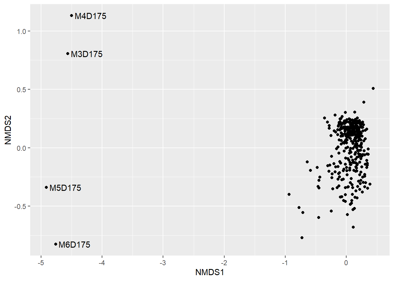
outliers <- names(which(bc.nmds$points[,1] < (-2)))
ps2.rare.sub <- subset_samples(ps2.rare, !sample_names(ps2.rare) %in% outliers)
ps2.rare.sub
## phyloseq-class experiment-level object
## otu_table() OTU Table: [ 179 taxa and 332 samples ]
## sample_data() Sample Data: [ 332 samples by 5 sample variables ]
## tax_table() Taxonomy Table: [ 179 taxa by 7 taxonomic ranks ]Now we’ve removed the outliers with respect to beta diversity from the analysis.
We need to restart the ordination with the outliers removed.
ord.meta <- data.frame(sample_data(ps2.rare.sub))
ord.asvs <- otu_table(ps2.rare.sub)
bc.nmds <- metaMDS(ord.asvs,
                   autotransform = F,
                   trymax = 30)
## Run 0 stress 0.166958
## Run 1 stress 0.1672417
## ... Procrustes: rmse 0.002291094 max resid 0.03849656
## Run 2 stress 0.1669582
## ... Procrustes: rmse 0.0002360357 max resid 0.003420412
## ... Similar to previous best
## Run 3 stress 0.168862
## Run 4 stress 0.166965
## ... Procrustes: rmse 0.0005240002 max resid 0.008058722
## ... Similar to previous best
## Run 5 stress 0.1669622
## ... Procrustes: rmse 0.0005768518 max resid 0.009724019
## ... Similar to previous best
## Run 6 stress 0.1669616
## ... Procrustes: rmse 0.0005699644 max resid 0.009642975
## ... Similar to previous best
## Run 7 stress 0.1669627
## ... Procrustes: rmse 0.0005786757 max resid 0.009679927
## ... Similar to previous best
## Run 8 stress 0.1688668
## Run 9 stress 0.1683744
## Run 10 stress 0.16742
## ... Procrustes: rmse 0.004168486 max resid 0.07423793
## Run 11 stress 0.1669691
## ... Procrustes: rmse 0.0006471376 max resid 0.007913315
## ... Similar to previous best
## Run 12 stress 0.1672501
## ... Procrustes: rmse 0.002280951 max resid 0.0375698
## Run 13 stress 0.1669582
## ... Procrustes: rmse 0.0001210431 max resid 0.001760401
## ... Similar to previous best
## Run 14 stress 0.1669651
## ... Procrustes: rmse 0.0004546973 max resid 0.005718155
## ... Similar to previous best
## Run 15 stress 0.1688696
## Run 16 stress 0.1669629
## ... Procrustes: rmse 0.0006064841 max resid 0.009749018
## ... Similar to previous best
## Run 17 stress 0.1672445
## ... Procrustes: rmse 0.002208099 max resid 0.03690399
## Run 18 stress 0.1669627
## ... Procrustes: rmse 0.0006047666 max resid 0.009768097
## ... Similar to previous best
## Run 19 stress 0.1688768
## Run 20 stress 0.166962
## ... Procrustes: rmse 0.0005992686 max resid 0.009660375
## ... Similar to previous best
## *** Solution reachedbc.pcoa <- ordinate(ord.asvs, method = 'PCoA')
# Calculate distance matrices
bc.dist <- metaMDSredist(bc.nmds)
bc.envfit.nmds <- envfit(bc.nmds ~ time + sex,
data = ord.meta,
display = 'sites',
na.rm = T)
bc.envfit.pcoa <- envfit(bc.pcoa$vectors[,1:2] ~ time + sex,
data = ord.meta,
display = 'sites',
na.rm = T)
# Extract fit data
# NMDS data
# Use ggvegan to extract the nmds data for plotting as ggplot object
bc.envfit.nmds.fort <- fortify(bc.envfit.nmds)
centroids.nmds <- subset(bc.envfit.nmds.fort, Type == 'Centroid')
centroids.nmds$Label <- c('early', 'midearly', 'mid', 'late', 'post',
'female', 'male')
vectors.nmds <- subset(bc.envfit.nmds.fort, Type == 'Vector')
# Get ellipse data
# Ellipse function
veganCovEllipse<-function (cov, center = c(0, 0), scale = 1, npoints = 100)
{
theta <- (0:npoints) * 2 * pi/npoints
Circle <- cbind(cos(theta), sin(theta))
t(center + scale * t(Circle %*% chol(cov)))
}
bc.nmds.df <- data.frame(MDS1 = bc.nmds$points[,1],
MDS2 = bc.nmds$points[,2],
time = ord.meta$time)
plot.new()
bc.nmds.ellipse <- ordiellipse(bc.nmds,
ord.meta$time,
kind = "sd",
conf = 0.95,
object = T)## Warning in plot.xy(xy.coords(x, y), type = type, ...): "object" is not a
## graphical parameter
## Warning in plot.xy(xy.coords(x, y), type = type, ...): "object" is not a
## graphical parameter
## Warning in plot.xy(xy.coords(x, y), type = type, ...): "object" is not a
## graphical parameter
## Warning in plot.xy(xy.coords(x, y), type = type, ...): "object" is not a
## graphical parameter
## Warning in plot.xy(xy.coords(x, y), type = type, ...): "object" is not a
## graphical parameter
summary(bc.nmds.ellipse)## early midearly mid late post
## NMDS1 0.27679173 -0.05190089 -0.12725344 -0.18871119 -0.2382166
## NMDS2 0.02737381 0.11750573 -0.09450458 -0.06479793 -0.1773802
## Area 1.28695458 0.71163846 0.23483242 0.15522114 0.5202201bc.nmds.ellipse.df <- data.frame()
for(tp in levels(ord.meta$time)){
bc.nmds.ellipse.df <- rbind(bc.nmds.ellipse.df,
cbind(as.data.frame(with(bc.nmds.df[bc.nmds.df$time==tp,],
veganCovEllipse(bc.nmds.ellipse[[tp]]$cov,
bc.nmds.ellipse[[tp]]$center,
bc.nmds.ellipse[[tp]]$scale)))
,time=tp))
}
# PCoA data
bc.envfit.pcoa.fort <- fortify(bc.envfit.pcoa)
centroids.pcoa <- subset(bc.envfit.pcoa.fort, Type == 'Centroid')
centroids.pcoa$Label <- c('early', 'midearly', 'mid', 'late', 'post',
'female', 'male')
# vectors.pcoa <- subset(bc.envfit.pcoa.fort, Type == 'Vector')
ord.bray.nmds.plot <- plot_ordination(
ps2.rare,
bc.nmds,
color = primary,
shape = secondary) +
theme_cowplot() +
scale_color_manual(values = primary_color_list) +
background_grid(major = 'xy', minor = 'none') +
coord_fixed(ratio = 1)
ord.bray.nmds.plot +
geom_label(aes(label = Label,
x = NMDS1,
y = NMDS2,
alpha = 0.90),
show.legend = F,
data = centroids.nmds,
inherit.aes = F) 
centroids.nmds <- subset(centroids.nmds,!centroids.nmds$Label %in% c('female',
                                                                     'male'))
ord.bray.nmds.plot +
  geom_label(aes(label = Label,
                 x = NMDS1,
                 y = NMDS2,
                 alpha = 0.90),
             show.legend = F,
             data = centroids.nmds,
inherit.aes = F) 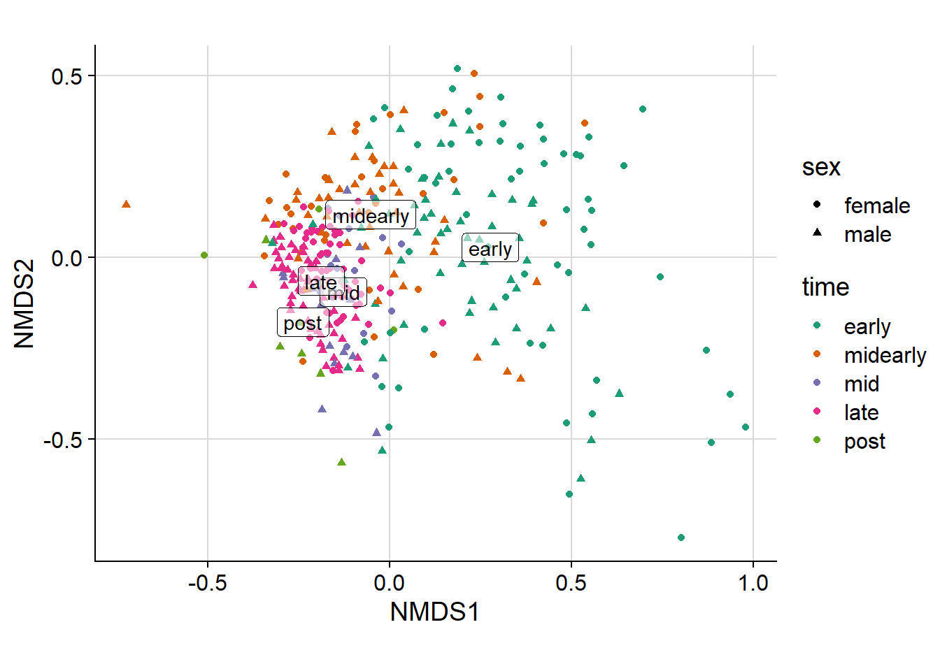
ord.bray.nmds.plot +
  background_grid(major = 'none', minor = 'none') +
  geom_path(data = bc.nmds.ellipse.df,
            aes(x = NMDS1, y = NMDS2, color = time),
            size = 1,
            linetype = 2,
inherit.aes = F) 
#   geom_segment(data = vectors.nmds,
#                aes(x = 0,
#                    y = 0,
#                    xend = NMDS1,
#                    yend = NMDS2),
#                arrow = arrow(length = unit(0.1, 'cm')),
#                color = 'black',
#                inherit.aes = F)

bc.envfit.nmds
##
## ***FACTORS:
##
## Centroids:
## NMDS1 NMDS2
## timeearly 0.2768 0.0274
## timemidearly -0.0519 0.1175
## timemid -0.1273 -0.0945
## timelate -0.1887 -0.0648
## timepost -0.2382 -0.1774
## sexfemale 0.0531 0.0319
## sexmale -0.0537 -0.0323
##
## Goodness of fit:
## r2 Pr(>r)
## time 0.3891 0.001 ***
## sex 0.0321 0.001 ***
## ---
## Signif. codes: 0 '***' 0.001 '**' 0.01 '*' 0.05 '.' 0.1 ' ' 1
## Permutation: free
## Number of permutations: 999# PERMANOVA
# Tests for differences in means of the data
bc.adonis <- adonis(bc.dist ~ time * sex,
data = ord.meta)
bc.adonis##
## Call:
## adonis(formula = bc.dist ~ time * sex, data = ord.meta)
##
## Permutation: free
## Number of permutations: 999
##
## Terms added sequentially (first to last)
##
## Df SumsOfSqs MeanSqs F.Model R2 Pr(>F)
## time 4 6.2082 1.55204 24.437 0.22065 0.001 ***
## sex 1 0.8273 0.82731 13.026 0.02940 0.001 ***
## time:sex 4 0.6496 0.16240 2.557 0.02309 0.001 ***
## Residuals 322 20.4510 0.06351 0.72686
## Total 331 28.1361 1.00000
## ---
## Signif. codes: 0 '***' 0.001 '**' 0.01 '*' 0.05 '.' 0.1 ' ' 1# TukeyHSD on Beta dispersions
# Tests for homogeneity of the data
bc.disper <- betadisper(bc.dist, ord.meta$time)
TukeyHSD(bc.disper)## Tukey multiple comparisons of means
## 95% family-wise confidence level
##
## Fit: aov(formula = distances ~ group, data = df)
##
## $group
## diff lwr upr p adj
## midearly-early -0.048222855 -0.071418402 -0.0250273075 0.0000003
## mid-early -0.081716911 -0.112961097 -0.0504727252 0.0000000
## late-early -0.102897239 -0.123663070 -0.0821314078 0.0000000
## post-early -0.054638352 -0.107909582 -0.0013671207 0.0412433
## mid-midearly -0.033494057 -0.066433120 -0.0005549937 0.0440902
## late-midearly -0.054674384 -0.077912337 -0.0314364315 0.0000000
## post-midearly -0.006415497 -0.060698153 0.0478671590 0.9976035
## late-mid -0.021180327 -0.052456008 0.0100953532 0.3425020
## post-mid 0.027078560 -0.031100238 0.0852573574 0.7057337
## post-late 0.048258887 -0.005030822 0.1015485961 0.0967398Let’s generate some barplots next
ps2.bar <- subset_samples(ps2.comp, !sample_names(ps2.comp) %in% outliers)

# Basic phyloseq plot
plot_bar(ps2.bar, fill = 'Phylum', x = primary) +
    geom_bar(aes(color = Phylum),
             stat='identity',
             position='stack')
# Merged phyloseq plot (100% total abundance)
ps2.bar.merge <- merge_samples(ps2.bar, group = primary)
## Warning in asMethod(object): NAs introduced by coercionsample_data(ps2.bar.merge)$time <- sample_names(ps2.bar.merge)
ps2.bar.merge.comp <- transform_sample_counts(ps2.bar.merge,
function(x) x/sum(x) * 100)
plot_bar(ps2.bar.merge.comp, fill = 'Phylum', x = primary) +
geom_bar(aes(color = Phylum),
stat='identity',
position='stack')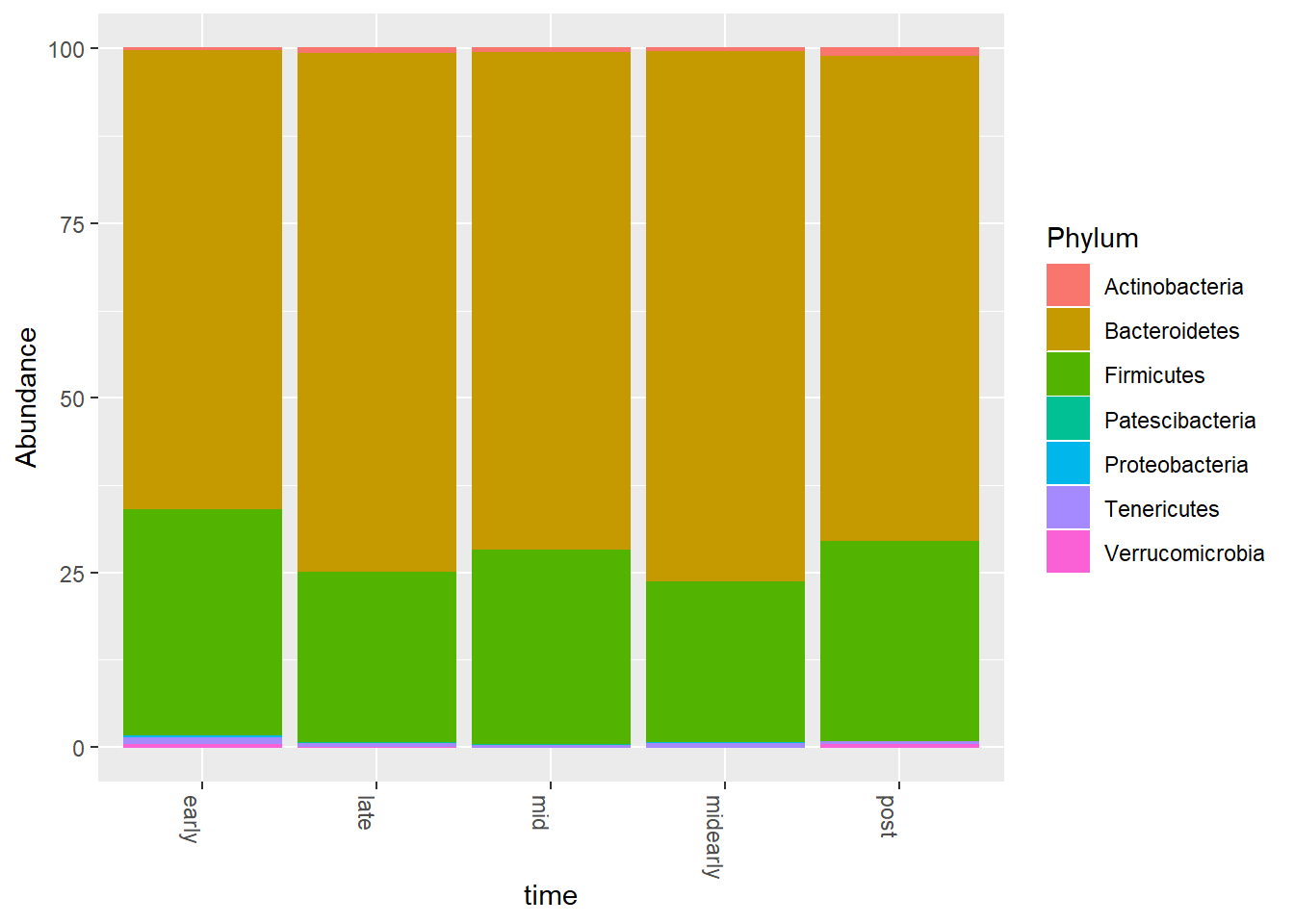
# Fully modified phyloseq plot
ps2.bp.phylum <- tax_glom(ps2.bar.merge.comp, 'Phylum', NArm = F)

taxa_count <- length(unique(tax_table(ps2.bp.phylum)[,'Phylum']))
getPalette <- colorRampPalette(brewer.pal(9, "Set1"))
cabd <- sort(taxa_sums(ps2.bp.phylum)/nsamples(ps2.bp.phylum),
             decreasing = T)
taxa_order <- as.character(tax_table(ps2.bp.phylum)[names(rev(cabd)), 'Phylum'])
taxa_order <- unique(taxa_order)
sample_order <- sample_names(ps2.bp.phylum)
bp.phylum <- plot_bar(ps2.bp.phylum, fill = 'Phylum') +
  geom_bar(aes(color=Phylum),
           stat='identity',
           position='stack') +
  scale_fill_manual(values = rev(getPalette(taxa_count))) +
  scale_color_manual(name = 'Phylum',
                     values = rev(getPalette(taxa_count))) +
  ylim(c(0,101)) +
  theme_cowplot() +
  xlab('timepoint')
bp.phylum$data[,'Phylum'] <- factor(bp.phylum$data[,'Phylum'],
                                    levels = taxa_order)
bp.phylum$data[,'Sample'] <- factor(bp.phylum$data[,'Sample'],
       levels = sample_order)
bp.phylum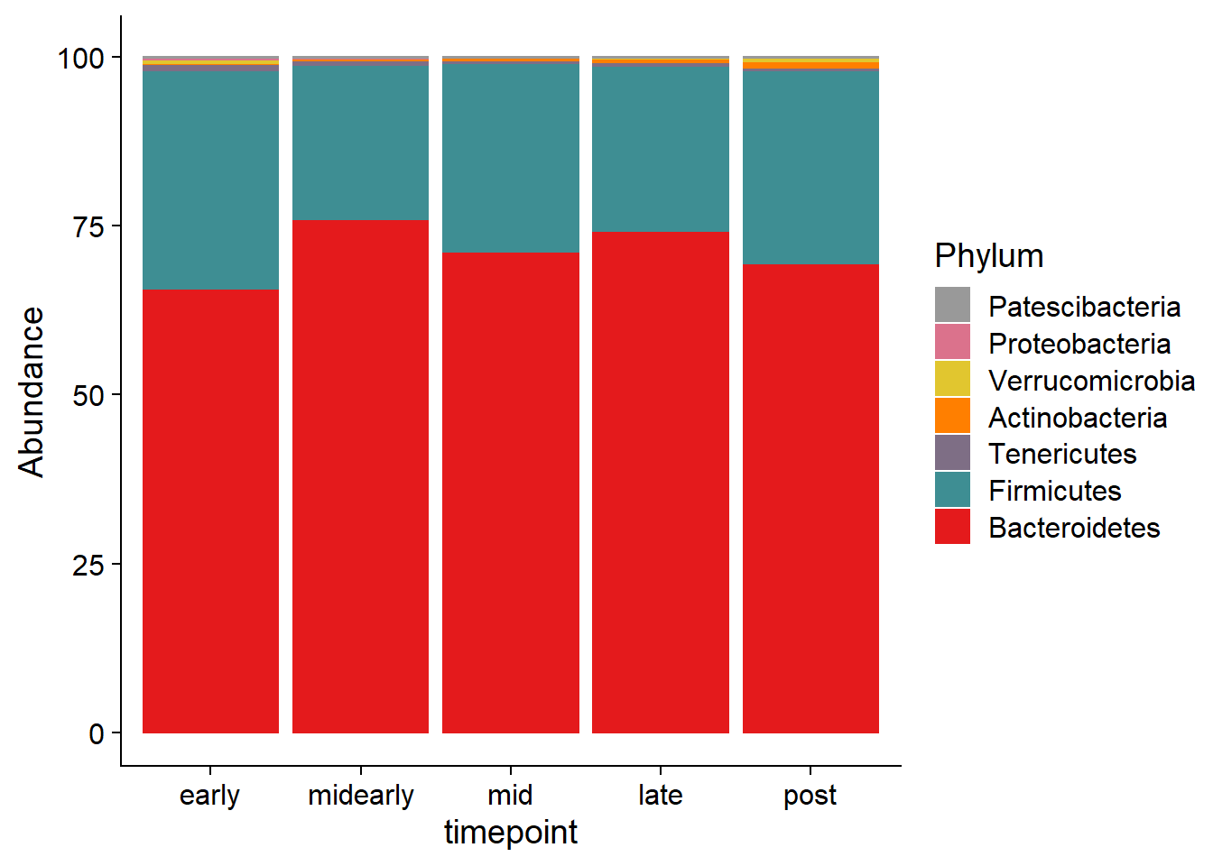
# Let's look at families
ps2.bp.family <- tax_glom(ps2.bar.merge.comp, 'Family', NArm = F)
ps2.bp.family
## phyloseq-class experiment-level object
## otu_table() OTU Table: [ 23 taxa and 5 samples ]
## sample_data() Sample Data: [ 5 samples by 5 sample variables ]
## tax_table() Taxonomy Table: [ 23 taxa by 7 taxonomic ranks ]cabd <- sort(taxa_sums(ps2.bp.family)/nsamples(ps2.bp.family),
decreasing = T)
# Lets remove some low abundance families
renamed.family <- names(which(cabd < 0.5))
tax_table(ps2.bp.family)[renamed.family, 'Family'] <- '< 0.5% Abd'
ps2.bp.family <- tax_glom(ps2.bp.family, 'Family', NArm = F)
cabd <- sort(taxa_sums(ps2.bp.family)/nsamples(ps2.bp.family),
decreasing = T)
taxa_count <- length(unique(tax_table(ps2.bp.family)[,'Family']))
getPalette <- colorRampPalette(brewer.pal(9, "Set1"))
taxa_order <- as.character(tax_table(ps2.bp.family)[names(rev(cabd)), 'Family'])
taxa_order <- unique(taxa_order)
sample_order <- sample_names(ps2.bp.family)
bp.family <- plot_bar(ps2.bp.family, fill = 'Family') +
geom_bar(aes(color=Family),
stat='identity',
position='stack') +
scale_fill_manual(values = rev(getPalette(taxa_count))) +
scale_color_manual(name = 'Family',
values = rev(getPalette(taxa_count))) +
ylim(c(0,101)) +
theme_cowplot() +
xlab('timepoint')
bp.family$data[,'Family'] <- factor(bp.family$data[,'Family'],
levels = taxa_order)
bp.family$data[,'Sample'] <- factor(bp.family$data[,'Sample'],
levels = sample_order)
bp.family
# ampvis2
#Combine OTU abundance table and taxonomy table from the phyloseq object "my_phyloseq_object":
av2_otutable <- data.frame(OTU = rownames(t(phyloseq::otu_table(ps2.bar)@.Data)),
                       t(phyloseq::otu_table(ps2.bar)@.Data),
                       phyloseq::tax_table(ps2.bar)@.Data,
                       check.names = F
)

#Extract metadata from the phyloseq object:
av2_metadata <- data.frame(phyloseq::sample_data(ps2.bar),
                       check.names = F
)

av2_metadata <- cbind(rownames(av2_metadata), av2_metadata)

#Load the data with amp_load:
av2_obj <- amp_load(av2_otutable, av2_metadata)
av2_box <- amp_boxplot(av2_obj, group_by = primary,
            sort_by = 'mean', tax_show = 10,
            tax_aggregate = 'Phylum',
            order_group = primary_order_list,
            normalise = F) +
  scale_color_manual(values = rev(primary_color_list))
av2_box
av2_box <- amp_boxplot(av2_obj, group_by = primary,
            sort_by = 'mean', tax_show = 10,
            tax_aggregate = 'Family',
            order_group = primary_order_list,
            normalise = F) +
  scale_color_manual(values = rev(primary_color_list))
av2_box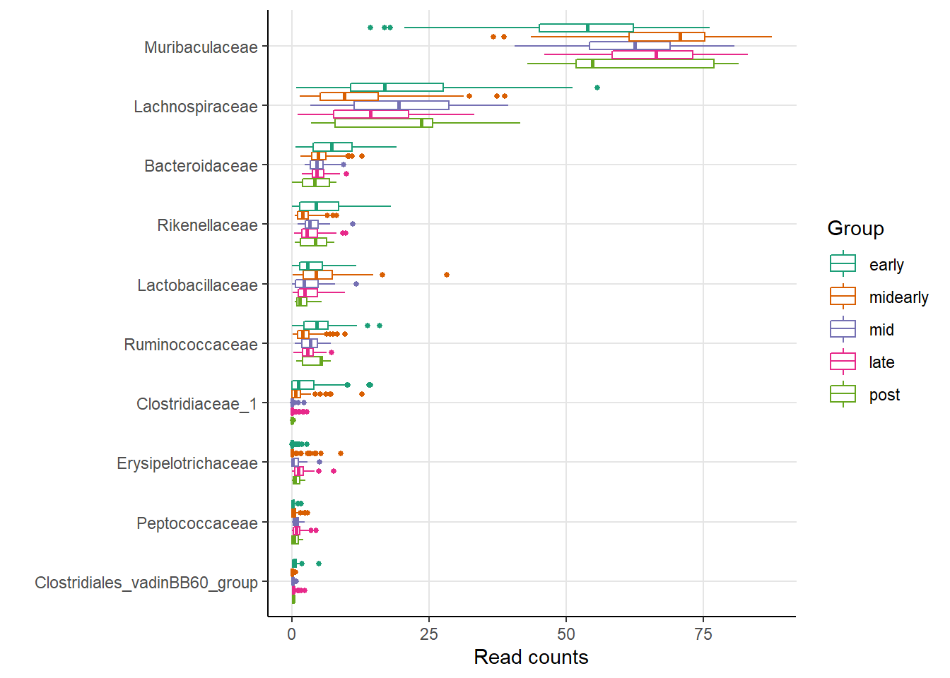
av2_box <- amp_boxplot(av2_obj, group_by = primary,
            sort_by = 'mean', tax_show = 10,
            tax_aggregate = 'Genus',
            order_group = primary_order_list,
            normalise = F) +
  scale_color_manual(values = rev(primary_color_list))
av2_box
# Use UpSetR to generate upset plots (Venn diagram alternative)
ps2.venn <- merge_samples(ps2.rare.sub, primary, fun = sum)
## Warning in asMethod(object): NAs introduced by coercionvenn_obj <- as.data.frame(t(otu_table(ps2.venn)))
venn_obj.binary <- sapply(venn_obj, function(x) ifelse(x > 0, 1, 0),
USE.NAMES = T)
rownames(venn_obj.binary) <- rownames(venn_obj)
venn_obj.binary <- as.data.frame(venn_obj.binary)
upset_order <- colnames(venn_obj.binary)
shared_ASV_plot <- upset(venn_obj.binary, nsets = 6,
sets = rev(upset_order),
mainbar.y.label = 'Shared ASVs',
sets.x.label = 'ASVs per Group',
keep.order = T,
order.by = 'freq', sets.bar.color = rev(primary_color_list))
shared_ASV_plot
R-session Information:
capture.output(sessionInfo())## [1] "R version 3.6.1 (2019-07-05)"
## [2] "Platform: x86_64-w64-mingw32/x64 (64-bit)"
## [3] "Running under: Windows 10 x64 (build 18362)"
## [4] ""
## [5] "Matrix products: default"
## [6] ""
## [7] "locale:"
## [8] "[1] LC_COLLATE=English_United States.1252 "
## [9] "[2] LC_CTYPE=English_United States.1252 "
## [10] "[3] LC_MONETARY=English_United States.1252"
## [11] "[4] LC_NUMERIC=C "
## [12] "[5] LC_TIME=English_United States.1252 "
## [13] ""
## [14] "attached base packages:"
## [15] "[1] stats graphics grDevices utils datasets methods base "
## [16] ""
## [17] "other attached packages:"
## [18] " [1] ggvegan_0.1-0 ggpubr_0.2.3 magrittr_1.5 "
## [19] " [4] UpSetR_1.4.0 ampvis2_2.5.4 here_0.1 "
## [20] " [7] cowplot_1.0.0 RColorBrewer_1.1-2 vegan_2.5-6 "
## [21] "[10] lattice_0.20-38 permute_0.9-5 ggplot2_3.2.1 "
## [22] "[13] phyloseq_1.30.0 dada2_1.14.0 Rcpp_1.0.1 "
## [23] ""
## [24] "loaded via a namespace (and not attached):"
## [25] " [1] nlme_3.1-140 bitops_1.0-6 "
## [26] " [3] matrixStats_0.55.0 lubridate_1.7.4 "
## [27] " [5] httr_1.4.0 doParallel_1.0.15 "
## [28] " [7] rprojroot_1.3-2 GenomeInfoDb_1.22.0 "
## [29] " [9] tools_3.6.1 backports_1.1.4 "
## [30] "[11] R6_2.4.0 lazyeval_0.2.2 "
## [31] "[13] BiocGenerics_0.32.0 mgcv_1.8-28 "
## [32] "[15] colorspace_1.4-1 ade4_1.7-13 "
## [33] "[17] withr_2.1.2 gridExtra_2.3 "
## [34] "[19] tidyselect_0.2.5 compiler_3.6.1 "
## [35] "[21] cli_1.1.0 Biobase_2.46.0 "
## [36] "[23] network_1.15 plotly_4.9.0 "
## [37] "[25] DelayedArray_0.12.0 labeling_0.3 "
## [38] "[27] bookdown_0.13 scales_1.0.0 "
## [39] "[29] stringr_1.4.0 ggnet_0.1.0 "
## [40] "[31] digest_0.6.21 Rsamtools_2.2.0 "
## [41] "[33] rmarkdown_1.15 XVector_0.26.0 "
## [42] "[35] base64enc_0.1-3 pkgconfig_2.0.2 "
## [43] "[37] htmltools_0.3.6 htmlwidgets_1.3 "
## [44] "[39] rlang_0.4.0 hwriter_1.3.2 "
## [45] "[41] jsonlite_1.6 BiocParallel_1.20.0 "
## [46] "[43] dplyr_0.8.3 RCurl_1.95-4.12 "
## [47] "[45] GenomeInfoDbData_1.2.2 biomformat_1.14.0 "
## [48] "[47] Matrix_1.2-17 munsell_0.5.0 "
## [49] "[49] S4Vectors_0.24.0 Rhdf5lib_1.8.0 "
## [50] "[51] ape_5.3 lifecycle_0.1.0 "
## [51] "[53] stringi_1.4.3 yaml_2.2.0 "
## [52] "[55] MASS_7.3-51.4 SummarizedExperiment_1.16.0"
## [53] "[57] zlibbioc_1.32.0 rhdf5_2.30.0 "
## [54] "[59] plyr_1.8.4 grid_3.6.1 "
## [55] "[61] parallel_3.6.1 ggrepel_0.8.1 "
## [56] "[63] crayon_1.3.4 Biostrings_2.54.0 "
## [57] "[65] splines_3.6.1 multtest_2.42.0 "
## [58] "[67] zeallot_0.1.0 knitr_1.23 "
## [59] "[69] pillar_1.4.2 igraph_1.2.4.1 "
## [60] "[71] GenomicRanges_1.38.0 ggsignif_0.6.0 "
## [61] "[73] reshape2_1.4.3 codetools_0.2-16 "
## [62] "[75] stats4_3.6.1 glue_1.3.1 "
## [63] "[77] evaluate_0.14 ShortRead_1.44.0 "
## [64] "[79] blogdown_0.15 latticeExtra_0.6-28 "
## [65] "[81] remotes_2.1.0 data.table_1.12.2 "
## [66] "[83] RcppParallel_4.4.4 vctrs_0.2.0 "
## [67] "[85] foreach_1.4.7 tidyr_1.0.0 "
## [68] "[87] gtable_0.3.0 purrr_0.3.2 "
## [69] "[89] assertthat_0.2.1 xfun_0.11.1 "
## [70] "[91] mime_0.7 viridisLite_0.3.0 "
## [71] "[93] survival_2.44-1.1 tibble_2.1.3 "
## [72] "[95] iterators_1.0.12 GenomicAlignments_1.22.0 "
## [73] "[97] IRanges_2.20.0 cluster_2.1.0 "
## [74] "[99] ellipsis_0.2.0.1 "